Visualization

This visualization tutorial uses an instance tok and sol obtained by fitting the tutorial data according to Getting Started.

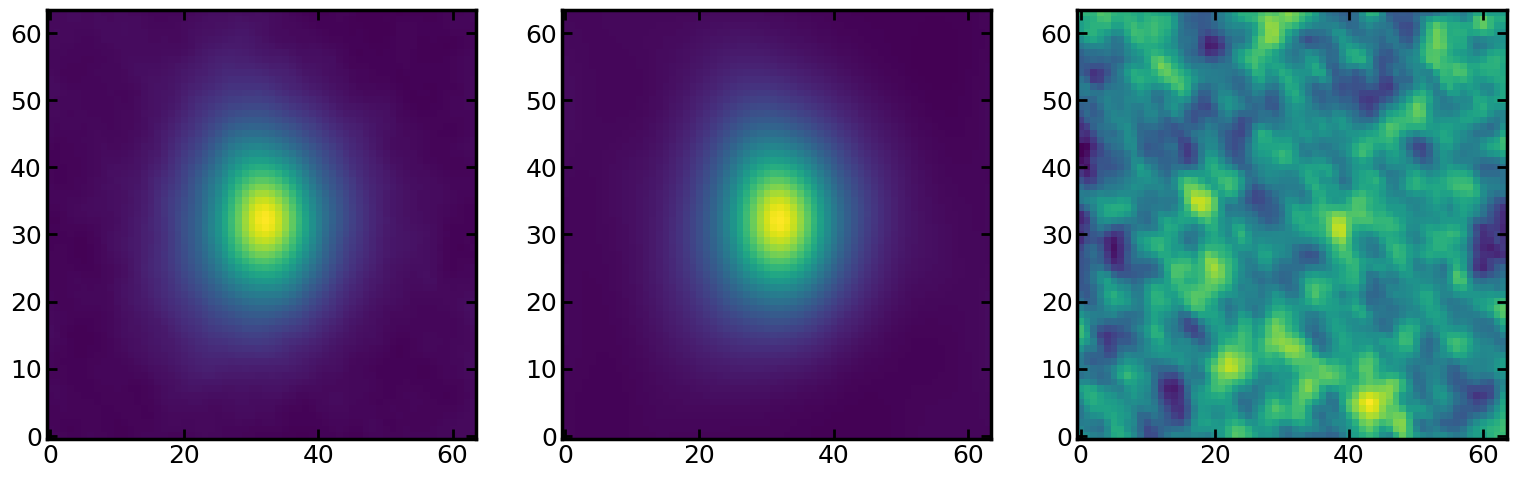
Moment 0 map

Cube.moment0() reutrns the moment-0 (integrated-flux) map of the data cube. The best-fit model cube is stored in the tok as tok.modelcube. We can visually compare the data and model using tok.datacube and tok.modelcube.

import matplotlib.pyplot as plt

fig, axes = plt.subplots(1, 3, figsize=[6.28 * 3, 6.28])
axes[0].imshow(tok.datacube.moment0(), origin='lower')
axes[1].imshow(tok.modelcube.moment0(), origin='lower')
axes[2].imshow(tok.datacube.moment0() - tok.modelcube.moment0(), origin='lower')

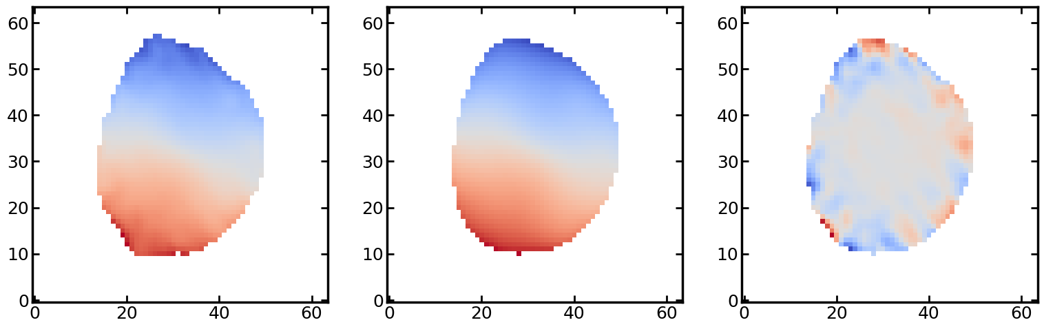
Moment 1 map

Similar to the moment-0 map, DataCube.pixmoment1() reutrns the moment-1 (velocity) map of the data cube.

import matplotlib.pyplot as plt

thresh = 3 * tok.datacube.rms_moment0()
v_center = np.nanmean(tok.datacube.pixmoment1(thresh=thresh))
m1_data = tok.datacube.pixmoment1(thresh=thresh) - v_center
m1_model = tok.modelcube.pixmoment1(thresh=thresh) - v_center

fig, axes = plt.subplots(1, 3, figsize=[6.28 * 3, 6.28])
axes[0].imshow(m1_data, origin='lower', cmap='coolwarm')
axes[1].imshow(m1_model, origin='lower', cmap='coolwarm')
axes[2].imshow(m1_data - m1_model, origin='lower', cmap='coolwarm')

Cube animation

There are several ways (including those not written in this section) to illustrate a 3D cube on python.

On the plot viewer, you can use matplotlib.pyplot.pause() to make animation of a 3D cube. This example shows the flux maps along the velocity axis.

import matplotlib.pyplot as plt

interval = 0.05
vsize = tok.datacube.vlim[1] - tok.datacube.vlim[0]
data = tok.datacube.imageplane

fig = plt.figure()
for i in range(vsize):
      plt.imshow(data[i, :, :], origin='lower', vmin=data.min(), vmax=data.max())
      plt.pause(interval)
      fig.clear()
      plt.clf()
plt.clf()
plt.close()

To save the animation in a file, matplotlib.animation is an option.

import matplotlib.pyplot as plt
import matplotlib.animation as animation

cube = tok.datacube.imageplane
vmin, vmax = cube.min(), cube.max()

fig = plt.figure(figsize=[6.28 * 0.7, 6.28 * 0.7])
ax = fig.add_subplot(1, 1, 1)
ims = []
for i in range(len(cube[:, 0, 0])):
    im = ax.imshow(cube[i, :, :], vmin=vmin, vmax=vmax, origin='lower')
    ims.append([im])

ani = animation.ArtistAnimation(
    fig, ims, interval=300, blit=False, repeat_delay=1000, repeat=True
)
ani.save('anime_cube.gif', writer='pillow')
plt.close()

…why does this animation have so poor image quality?

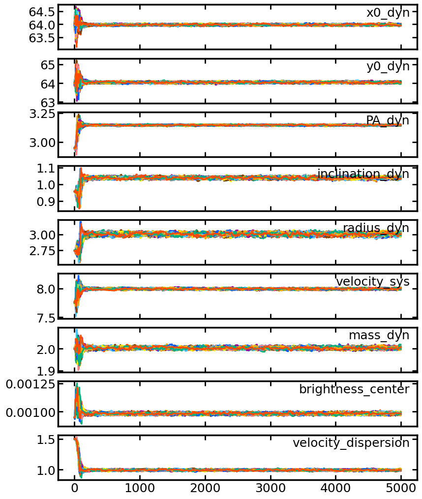
Convergence of MCMC sampler

The MCMC sampler during the MCMC fitting are stored in the solution, sol.sampler. You can check whether the MCMC fiting is converged using this attribute.

Note

Even if you performed fitting with the methods other than MCMC, there exists sol.sampler, but None is stored.

This code plots the behavior of the nine parameters at each step.

import matplotlib.pyplot as plt

samples = sol.sampler.get_chain()
label = sol.best._fields

fig, axes = plt.subplots(9, 1, figsize=[6.28 * 1.5, 6.28 * 2])
for i in range(9):
    axes[i].plot(samples[:, :, i])
    axes[i].text(0.98, 0.95, label[i], ha='right', va='top', transform = axes[i].transAxes)
    if i != 8:
        axes[i].xaxis.set_ticklabels('')

Tokult implement emcee as a MCMC sampler, so please see the emcee document for the details of how to manipulate the sampler.