Getting Started

Preparing Data

The tutorial data are provided in this url: https://github.com/sugayu/tokult/tree/dev/tutorial. Download the data and put them on a directory to work in. You can download the data from the terminal with:

$ svn export https://github.com/sugayu/tokult/branches/dev/tutorial/
$ cd tutorial

The donwloaded data are:

tokult_mockcube_dirty.fits

The ALMA mock dirty cube with natural weighting.

tokult_cube_dirty.psf.fits

The ALMA dirty beam with natural weighting.

tokult_cube_dirty_uniform.psf.fits

The ALMA dirty beam with uniform weighting.

tokult_x-arcsec-deflect.fits

The map of the deflection angles along the \(x\) axis.

tokult_y-arcsec-deflect.fits

The map of the deflection angles along the \(y\) axis.

tokult_gamma1.fits, tokult_gamma2.fits, tokult_kappa.fits

The gamma1, gamma2, and kappa lensing parameter maps. Not needed in this tutorial.

Quickstart

Launching a Tokult instance

First of all, import the Tokult package and then launch Tokult by inputting the file names.

import tokult

tok = tokult.Tokult.launch(
    'tokult_mockcube_dirty.fits',
    'tokult_cube_dirty.psf.fits',
    ('tokult_x-arcsec-deflect.fits', 'tokult_y-arcsec-deflect.fits'),
)

tok provides basic fitting modules of Tokult. The first argument takes the file name or the np.ndarray of the data cube, the second takes the dirty beam (point spread function), and the third takes the lensing parameters summarized in a tuple.

Next, Tokult needs to know which cubic region you want to use for the model fitting. The current code does not work without specifying the region. In addition, the lensing parameters (x-deflection and y-deflection) need redshifts of the lensing cluster and the target object; in this tutorial, the cluster and mock galaxy are assumed at z = 0.541 and z = 1.7, respectively. tok can take these parameters with the methods use_region() and use_redshifts().

tok.use_region(xlim=(32, 96), ylim=(32, 96), vlim=(5, 12))
tok.use_redshifts(z_lens=0.541, z_source=1.7)

The xlim, ylim, and vlim determine the size of an argument tok.datacube.imageplane and others. The redshift information is stored in internal parameters and also used to convert the parameters to those in physical units later.

uv-coverage

This step can be skipped if you use the image-plane fitting. The current uv-plane fitting requires a re-sampled uv coverage of the observations. The uv coverage can be obtained from a dirty beam created with uniform weighting.

import numpy as np
from astropy.io import fits

data = fits.getdata('tokult_cube_dirty_uniform.psf.fits')
uvpsf_uniform = tokult.misc.rfft2(np.squeeze(data))
uvcoverage = (uvpsf_uniform[tok.datacube.vslice, :, :]) > 1.0e-5  # This value 1.0e-5 is like arbitrary.

Here, uvcoverage is a mask, i.e., np.ndarray including Boolean; True indicates that the pixels are used in fitting and vice versa.

Setting/Guessing initial parameters and bounding

Initial parameters for fitting can be set by hand, or Tokult employs the method initialguess to estimate initial parameters from the moment-0 and 1 maps. Tokult also provides tokult.get_bound_params(), which makes it easy to specify the parameter boundaries.

init = tok.initialguess()
init = init._replace(mass_dyn=2.0)  # To fix a bug(?)
bound = tokult.get_bound_params(
    x0_dyn=(32, 96),
    y0_dyn=(32, 96),
    radius_dyn=(0.01, 5.0),
    velocity_sys=(5, 12),
    mass_dyn=(-2.0, 10.0),
    velocity_dispersion=(0.1, 3.0),
    brightness_center=(0.0, 1.0),
)

The fitting parameters are explained here [TBD].

Quick initial fitting

Now you are ready! First, let’s try to perform fitting on the image plane with the least-square method.

Note

The least-square method may fall in local minima if the initial parameters are far from the true values, but it is useful to know whether the fitting code works.

sol = tok.imagefit(init=init, bound=bound, optimization='ls')

Done. Let’s check the fitting results, which are contained in sol. The best fit parameters are contained in sol.best:

sol.best

InputParams(x0_dyn=63.98926461367171, y0_dyn=64.01280881181941, PA_dyn=3.1435523445232345, inclination_dyn=1.030729882664348, radius_dyn=2.9962304513969964, velocity_sys=7.996353444267494, mass_dyn=2.001782648183586, brightness_center=0.0009768938914882768, velocity_dispersion=0.9902675180818492, radius_emi=2.9962304513969964, x0_emi=63.98926461367171, y0_emi=64.01280881181941, PA_emi=3.1435523445232345, inclination_emi=1.030729882664348)

These output values are in units of pixels for simplicity in the code. The physical units are added by:

sol.add_units()

FitParamsWithUnits(x0_dyn=<Longitude 177.38993349 deg>, y0_dyn=<Latitude 22.41271684 deg>, PA_dyn=<Quantity 3.14355234 rad>, inclination_dyn=<Quantity 1.03072988 rad>, radius_dyn=<Quantity 0.14981152 arcsec>, velocity_sys=<Quantity -0.18232766 km / s>, mass_dyn=<Dex 2.00178265 dex(pix3)>, brightness_center=<Quantity 0.39075756 Jy / arcsec2>, velocity_dispersion=<Quantity 49.52163522 km / s>, radius_emi=<Quantity 0.14981152 arcsec>, x0_emi=<Longitude 177.38993349 deg>, y0_emi=<Latitude 22.41271684 deg>, PA_emi=<Quantity 3.14355234 rad>, inclination_emi=<Quantity 1.03072988 rad>)

The method add_units() makes use of the header information of the data and the lensing parameter map.

The best-fit result can be visualized by like this:

import matplotlib.pyplot as plt

fig, axes = plt.subplots(1, 3, figsize=[6.28 * 3, 6.28])
axes[0].imshow(tok.datacube.moment0(), origin='lower')
axes[1].imshow(tok.modelcube.moment0(), origin='lower')
axes[2].imshow(tok.datacube.moment0() - tok.modelcube.moment0(), origin='lower')

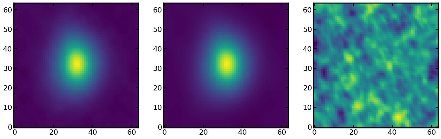
The left and middle panels show the moment-0 maps of the data and best-fit model, respectively. The data was well-reproduced by the model, and the residual map looks like pure noises as the right panel.

Restarting model-fit

It is known that the least-square method may underestimate the fitting uncertainties for the spatially-correlated data. To obtain correct uncertainties, as well as to escape from shallow local minima, the MCMC method on the uv plane is a great option.

Let’s fit an example data; but it takes more than the least-square method, maybe >~10 minutes for the tutorial data.

sol = tok.uvfit(
    init=init, bound=bound, mask_for_fit=uvcoverage, progressbar=True
)

100%|███████████████████████|5000/5000 [18:57<00:00,  4.40it/s]

If you want to use parallelization, please see [TBD].

Parallelization

Short code as an example.

import multiprocessing

with multiprocessing.Pool() as pool:
    sol = tok.uvfit(
        init=init,
        bound=bound,
        mask_for_fit=uvcoverage,
        progressbar=True,
        pool=pool
    )